Almost all the work that people do in offices is done with the help of a magical program called Microsoft Excel, when you first look at it it might look like a program with only tables and slots for entering data, but this description does not suffice for the real capability of this program. Excel can do anything from managing your office accounts to managing the data required for managing a whole country, you just need to know how to use it. Here in this article a few really cool Excel tips and tricks are mentioned that can help many users to improve the way in which they have used excel till date.
1. Adding Shortcuts To Top Menu
There are many tools that we always wish we had just a click away, but mostly we have to make more than a couple of clicks and also a bit of searching to get to the tool that we wish to get into use. If we look at the top left corner of our excel window, we’ll see a small excel icon, along which there will be 3 small icons, one of them representing Save, and the other 2 being undo and redo.

These are the shortcuts that excel provides for our ease, the other thing that excel provides is the option to put more shortcuts at this place. For this purpose, you need to click on an arrow to the right of undo and redo that says Customize Quick Access Toolbar when you hover over it.
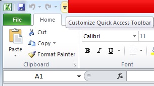
Pressing it will give you an option of selecting the tool that you wish to add to your quick access toolbar (the place on the top left where save, undo and redo are present). For instance, if we click on the ‘New’ option, we’ll get the icon to create a new file in our toolbar.

2. Adding Diagonal Lines
We can add diagonal lines in our cells by a simple method of formatting that excel allows. For this all we need to do is select a cell in which we wish to add a diagonal line, upon selecting the cell we would need to open the options by right clicking on the mouse. In the options we would need to click on the option of Format Cells.

When we click on the Format cells option, we’ll see a dialog box, in which we’ll need to click on the border option, highlighted by red, in the top strip. Then we can click on the other highlighted option that shows us the format of a diagonal line in the cell, there is another one in the dialog box that you can find on your own.

Pressing ok after selecting the diagonal line as the border style will create a diagonal line in the cell that we intended to put our diagonal line in. To add text above and below the diagonal line, we’ll need to enter something in the cell and then press Alt+Enter to take it to the next line, and then type something else in the second line that we need to have below our diagonal line. One catch here is that we’ll need to take care of the alignment of our text above and below the diagonal line using spacebar.
 3. Moving and Copying Data To and From Cells. (using drag and drop along with Ctrl)
Whenever we type something in a cell in excel, we can always cut it from one place to another by first right clicking on the cell and pressing on cut, and then pasting it in some other cell. Another efficient method to do the same is by using the method of drag and drop. All you need to do for this is, go on the cell that you wish to move, and place your cursor on the border of that cell, this will cause a symbol with 4 arrows pointing in all directions to come up( this symbol signifies that you can now select the cell and then move it wherever you wish to).
If you now click on this symbol and take your cursor to another cell while still pressing it, you’ll see that something is coming along with the cursor. So finally if you go to a different cell and let go of the cursor then you’ll see that the content of the cells would have moved to the new location.

Till now we discussed how we could move data from one cell to another, another function that we use quite a lot is the copy function. We can even perform a copy using this drag and drop method, but for that we would need to press Ctrl before clicking on the symbol that we talked about in the text above. This will cause a new symbol to come up as shown in the figure below. You can then keep your hold on the Ctrl key and then try dragging and dropping the cell somewhere else, you’ll see that this method copies the contents of the cell instead of moving it.

4. Restricting Input
What happens if we wanted only a specific set of values in our sheet, and a data value coming from outside of our intended range comes up? It happens to be an issue many times while working on projects, and this causes problems with the final outputs that we intend to get. In order to make sure that only a certain set of values is added, we take the help of data validation. What it does is that it allows us to restrict the range and the type of data that we take as input for our system.
For using the data validation function, one need to select the cells in which the restriction is to be implemented, then on the topmost strip we would need to click on data.

Upon clicking on data, we’ll need to click on Data validation as shown in the image. This will take us to the dialog box in which we can set the values that we want for our system. We will then need to select the type of input that we would like to allow in the selected cells by clicking on the allow option in the dialog box.


For instance, if we select whole numbers, then we would be asked to select the range of the whole numbers that we would like to allow. Doing this we would only be able to enter data in the range that we have mentioned. Taking an example, we take the range to be between 12 and 111.

In the example that we have taken, you can see that upon entering a value outside of this range, i.e. 222, we are getting an error that the value is invalid and a restriction has been placed by the user on the values that can be entered in this cell.
5. Getting More Statistics in the Bar at the Bottom
Whenever we use excel to enter data into our tables in the form of numbers, we see certain statistics or a kind of summary in the status bar below, usually it will carry the average, count and sum of the data that we select at any given point of time.
Excel gives us certain more options for the summary that we get in the status bar, to exploit it to the maximum, one can do this by right clicking anywhere on the status bar, once you right click on the status bar, you’ll see a lot of options among which would be the additional options that excel provides us for the summary of data that we have selected. We can choose from Average, Count, Numerical Count, Minimum, Maximum and Sum. In the image we can see how our status bar looks when we select to view most of the options available to us.

6. Transforming the Case (Uppercase, Lowercase) of the Text
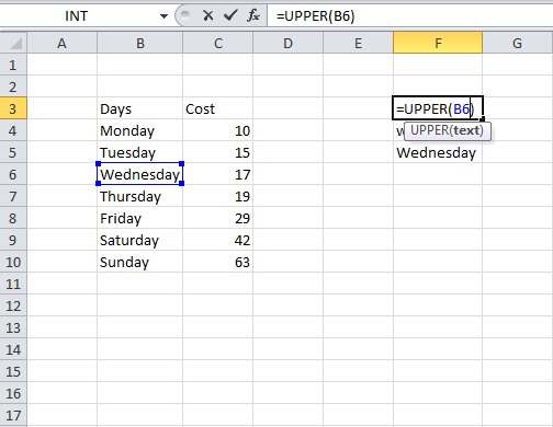
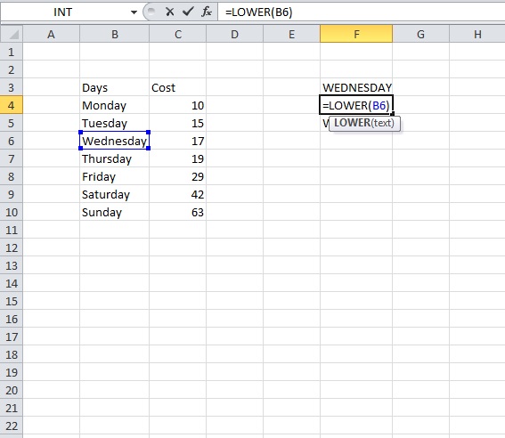
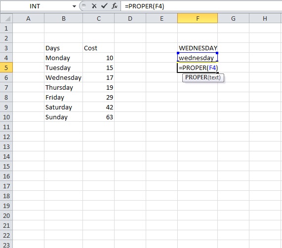
There is a small function that we can use to transform the case of our text, the function is quite easy to use, all you need to do for this is that you need to type ‘UPPER(text/cell)’ for upper case, ‘Lower(text/cell)’ for lower case and finally ‘Proper(text/cell)’ for making the first letter of the word capital. Its usage can be seen in the images below, with cells showing Upper, Lower and proper usage along with the final output that they achieve from it.
7. Arrange Text From Different Cells Using ‘&’
We can add text from different cells to a single cell by simply using ’&’, for this all we need to do is start writing in the cell with ‘=’ and then click on the cells one by one that we need to add to our new cell, we would also need to add’&’ after we click on each cell to be added, as it will add the name of the cell that we have clicked. So it will look something like the one in the image below.


8. Adding Multiple Rows or Columns At Once
We all know how to add a row or a column to our excel document, but what we also need to realize is that how we can actually add multiple rows or columns all at once instead of adding a column or a row at a time and then repeating the process again and again.
For this, first we’ll need to select the number of rows that we would like to add, for instance, if we need to add 4 new rows to our already existing table, then we’ll select 4 rows (below/above which we need to add rows) and then right click and click on insert. It will open up a small dialog box allowing us to select what exact action we need to perform on the rows/column selected.

If we press entire row in the dialog box, we’ll get 3 rows added inside our table. You can play around with the insert dialog box to see what other options have in store for you.

9. Using Auto-Correct
If you suffer from a habit of using SMS or in other words short hand language everywhere you type, or if you have a bad history of making spelling errors for some particular words, then you can use the auto-correct feature of MS Excel at your convenience. For using it you’ll first need to go to File>Options>Proofing>AutoCorrect Options. Here you’ll see a dialog box that will allow you to enter a text to be replaced with the text you would want to replace it with. You can add any words that you misspell, for example I can put ‘frnz’ as a word to be replaced by the word ‘friends’, and every time I use the wrong spelling(frnz), autocorrect will correct me(by putting friends in its place).

10. Extracting Web Page Data Using Data-> From Web
Ever wondered how it will feel to extract data straight out of a website, let’s say you see a website and you wish to analyze a particular thing from the data present on that particular webpage. For instance if we take a website with some faculty names on it and go on to turn this webpage directly into excel data using an online tool like this, what we’ll get is a table in with some converted data and finally we can download it as a .csv file to be viewed on excel, in the data that we have in the image below, we can look at all the data that we had on the website in a well-organized and tabulated form.
This technique can also be used for pages with enormous amounts of data, which we can then easily analyze on excel.
11. Creating Histogram of Data Using Data Analysis Option
For creating a histogram we’ll first of all need to add an add-in to our excel. For this purpose, you’ll first need to go to File>Options>Add-Ins. Once we see the add-ins window/options, we’ll need to make sure that Excel Add-Ins is selected in the Manage option near the lower end of the dialog box of options. There once we select Excel Add-Ins, we would need to select go to get a dialog box for Add-Ins. In that dialog box, we’ll need to check Analysis ToolPak and click OK.


Once we are done with the above prerequisites, we would need to go to the Data Analysis option in the analysis section under Data. Clicking on it will open a small dialog box named Data Analysis. In that dialog box we’ll need to select histogram and click OK. It will then ask us to put an input range of data on the basis of which we wish to create our histogram. We can then select the appropriate options to create the histogram that we wish to create.


12. Conditional Formatting
Conditional formatting is a powerful tool that excel incorporates, as the name suggests, conditional formatting formats cells on certain conditions, for instance, if we had to highlight the students who have failed in an exam in the class with red, then we would use conditional formatting.

For doing it we would need to select the cells to be formatted and then we’ll click on conditional formatting option and then we can click on new rule to make a new rule to be implemented on our data. In the example below, all roll numbers with marks between 0 and 40 will be marked with a red.

13. Using Fill Handle to Copy Formatting (Advanced Formatting)
A fill handle is a tool that shows us how nicely the software named excel is made, it is among the most easy to use tools in excel; still the kind of work it does is much more than many of the complicated tools that we have around. Just imagine how you would feel if you were told that you just need to format a single or two cells and all the other cells would be taken care of just by a click and a drag. What it does is that it looks for a pattern in the cells and then as you drag it, it fills the values it feels are appropriate.

For using the fill handle, you need to go to the bottom right corner of you cell or the selected cells, and you’ll see a solid ‘+’ . If you hold it and drag it, you’ll see the magic happening.
Now a number of options allowed with formatting with a fill handle are explained below.
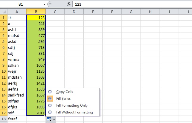
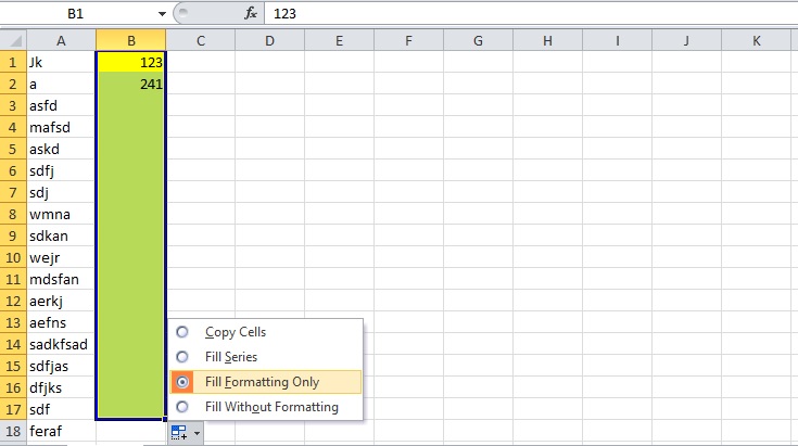
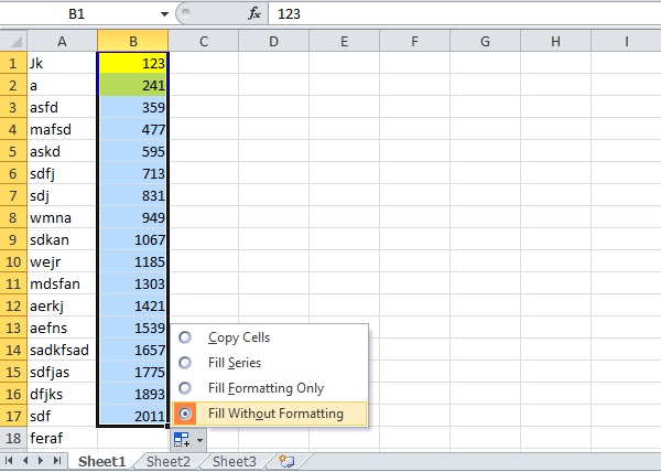
In the images below, you can see the options that you get upon filling certain cells using a fill handle; the options include Copy cells, Fill Series, Fill Formatting Only and Fill without Formatting. You can see what the latter 3 options do from the images accompanying this point.
14. Having a Live Transposed Copy of a Table
We know how to get a transposed copy of our data, if some of you don’t then don’t worry all you need to copy the data you want to transpose and then while pasting look for paste options and then click on transpose, you’ll get a transposed version. This being a kind of normal copy and paste operation will only create a fixed transposed version of the original table.
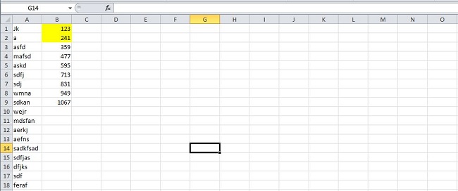
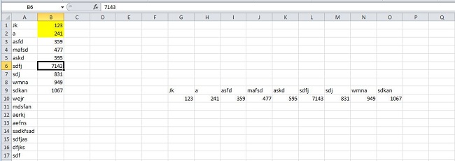
To make a live transposed version of your data, you’ll need to do a bit more than just copy and paste. For it first of all you’ll need to see how many rows and columns you have and then select a transposed version of those many columns and rows. For instance in the images below, you can see the data to be copied has 9 rows and 2 columns, and the area that we select after that has 9 columns and 2 rows.

Upon selecting these new columns and rows, you’ll need to type =Transpose(‘ coordinates of the Top Left corner of your data cells’ : ‘Coordinates of the bottom right corner of your data cells’), in the images below, they happen to be a1 and b9, so the equation to be entered becomes ‘=Transpose(A1:B9)’, upon entering this equation you’ll need to press ‘Shift+Ctrl+Enter’, and you’ll see the magic happen.

A new transposed table is thus created, but it is a live copy of the original one, i.e. if you make any changes to the original one, there will be changes to this table as well. As you can see in the images below, when the data in B6 is changed, data in L10 automatically changes. A small tradeoff is that you cannot copy the format that the data in original table had, and it is quite evident from the fact that 2 yellow cells didn’t carry their yellow color to the live transposed copies.
15. Entering Sparkline Microcharts
Sparkline microcharts are small graphs or charts that you can place in a cell. They were introduced in MS Word 2010 and can greatly enhance the view-ability of our excel data. To make one, you need to first select the data from which you wish to create a sparkline, and then go to Inset>Line.

There you would be asked to enter the destination location of your sparkline chart. Once you enter the destination you’ll a have beautiful sparkline chart waiting there for you.


SEE ALSO: 14 Cool Instagram Tips And Tricks
We hope this article helped you learn some really cool Excel tricks that you didn’t know about. If you have any query, feel free to ask in comments section.